How much water should remain in the Turag? It is a useful question, but the answer needs a place, a season, and a purpose. A flow that maintains a wetted channel may still leave habitat under stress. The timing and duration of low flow also matter.
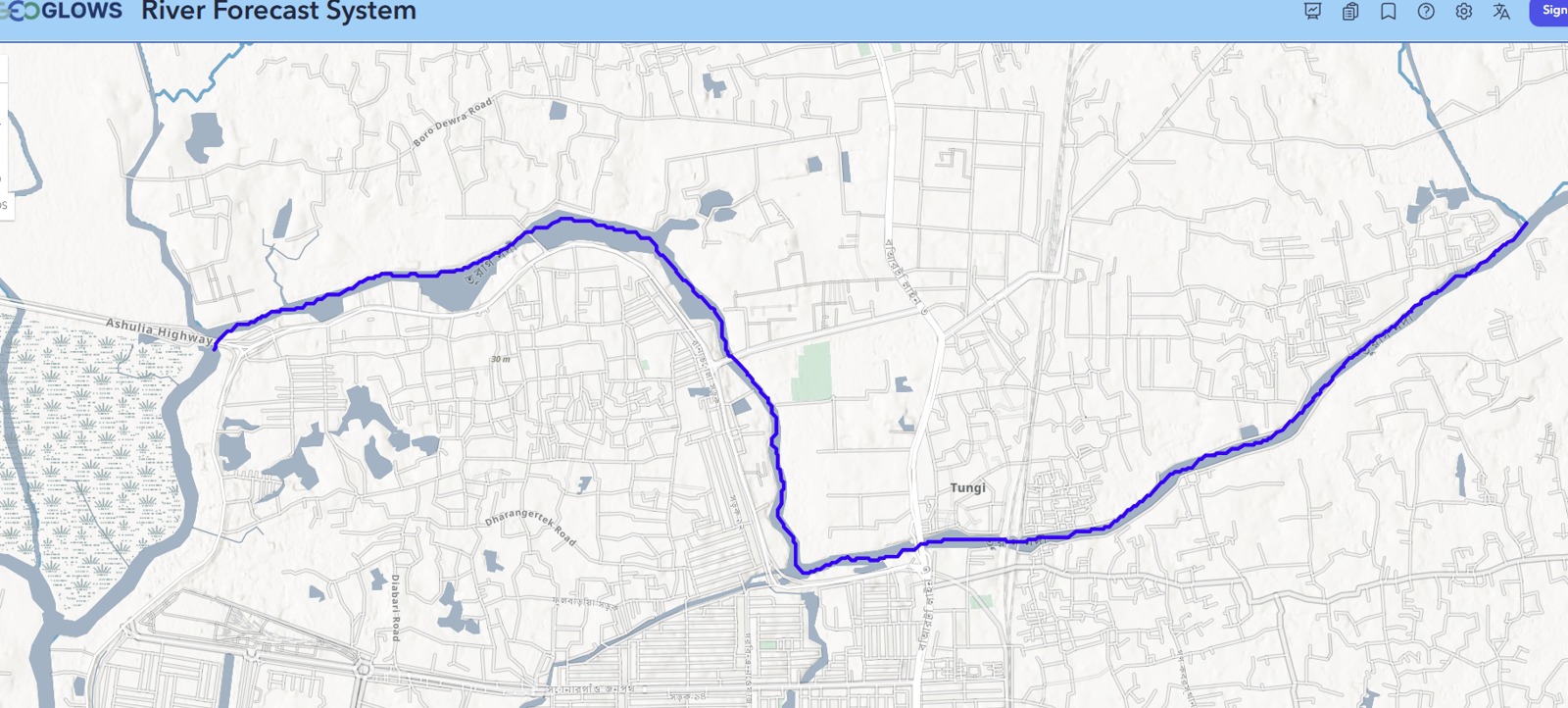
I combined my review of published Turag studies with an eight-scenario comparison of an archived 2006–2025 GEOGLOWS discharge series associated with the Tongi Bridge area near Uttara Diabari. Together, they show how to read environmental-flow numbers without losing the river behind them.
Why published estimates differ
Earlier Turag work uses different stations, records, and rules. Rahman and colleagues’ 2013 paper reported selected values of 206.50 m³/s for its Range of Variability Approach, 180.77 m³/s for its flow-duration approach, and 190.88 m³/s for its selected Tennant scenario. Those values belong to that study’s location and reference data. Applying them unchanged to a smaller connected reach would skip the questions that produced them.
| Method | What it summarizes | Question to ask |
|---|---|---|
| Tennant | A selected proportion of long-term mean flow | Which habitat scenario and seasonal coefficients were chosen? |
| Monthly allocation | A share of mean or median monthly flow | How were low and high months defined? |
| Flow duration curve (FDC) | The flow equaled or exceeded for a stated share of time | Does the quantile use the whole year or one season? |
| Range of Variability Approach (RVA) | Departure from reference flow characteristics | What baseline and target range were used? |
Q90 is an exceedance statistic. It represents a flow equaled or exceeded about 90% of the time in the selected record. The curve summarizes frequency; a separate timeline is needed to see whether low-flow days occurred together.
What the 20-year comparison shows
The archived series contains 7,305 daily modeled values for 2006–2025. Its mean is 19.51 m³/s. The first decade averages 20.38 m³/s and the second 18.64 m³/s, a descriptive reduction of 8.55%. Yet the annual trend test gives p = 0.319. The record therefore supports a difference between the two period averages, while providing limited evidence for a persistent annual trend.
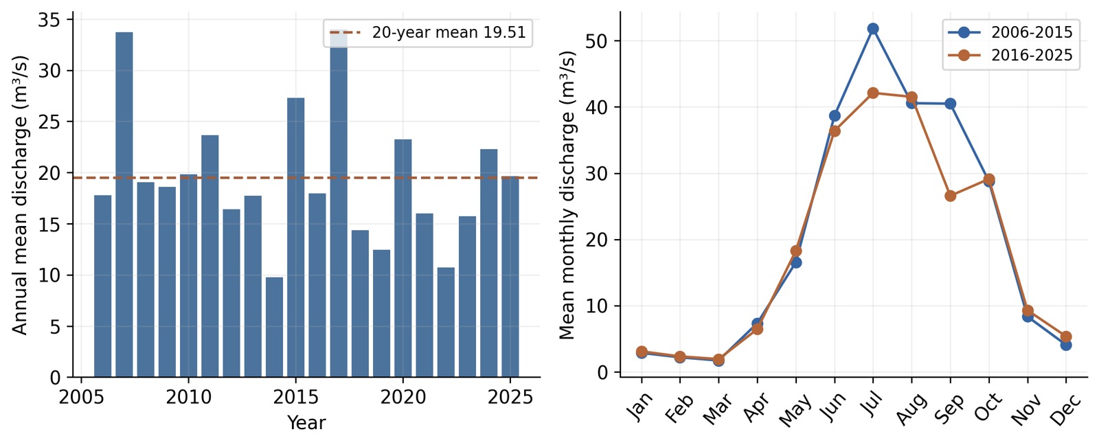
The seasonal picture is more informative than the annual average alone. Under the common low-flow month grouping used in the analysis, mean low-season flow rises by 5.64% between decades, while mean high-season flow falls by 10.44%. A lower annual mean can coexist with a higher dry-season mean.
Eight methods produce eight candidate schedules
The comparison includes Tennant good and fair scenarios, Tessmann, variable monthly flow, modified constant yield, two FDC schedules, and a moderate-status Smakhtin adaptation. Their annual mean thresholds range from 3.26 to 9.08 m³/s. Historical days below the chosen thresholds range from 15.29% to 47.28%.
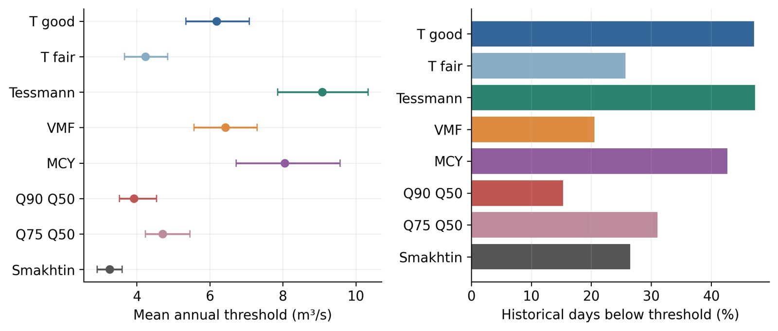
This spread is a finding about method choice. Selecting the smallest threshold would lower the apparent deficit, while selecting a larger one would increase it. A sensible choice needs a management objective and evidence about local depth, velocity, habitat, and water quality.
Combine flow and pollution evidence
Discharge is only one part of river condition. Wastewater load, dissolved oxygen, channel shape, backwater effects, and habitat connections also influence outcomes. Higher flow can change pollutant concentration, but treatment and source control remain necessary parts of river management.
For a local investigation, I would assemble discharge or stage observations, cross-sections, withdrawal records, seasonal water quality, and habitat observations. I would also record how long low-flow episodes last and when they occur. That turns a threshold into a question that can be checked on the river.
Use the results at the right scale
These are hydrological screening results from an archived model export. The export’s exact model-reach identifier and location-specific bias need confirmation before operational use. Published station values and model-reach values should retain their own labels. Local monitoring can then test which candidate seasonal schedule protects the functions people want to retain.
Sources and further reading
GEOGLOWS retrospective-data documentation explains the modeled discharge product. Ali and Hasan’s Gorai comparison provides the multi-method framework. Pastor and colleagues discuss environmental-flow methods. The literature review also uses Rahman et al. (2013), DOI 10.12983/ijsres-2013-p291-299, and the station-based preprint by Tasnim et al. (2023), DOI 10.22541/essoar.167326693.37637161/v1.
Continue reading
Diabari Waterlogging and Solid Waste Management · Diabari Wetlands, Drainage and Habitat Protection
Leave a Reply